42 rotate data labels excel chart

› documents › excelHow to group (two-level) axis labels in a chart in Excel? The Pivot Chart tool is so powerful that it can help you to create a chart with one kind of labels grouped by another kind of labels in a two-lever axis easily in Excel. You can do as follows: 1. Create a Pivot Chart with selecting the source data, and: (1) In Excel 2007 and 2010, clicking the PivotTable > PivotChart in the Tables group on the ... How to Use Cell Values for Excel Chart Labels - How-To Geek 12/03/2020 · Make your chart labels in Microsoft Excel dynamic by linking them to cell values. When the data changes, the chart labels automatically update. In this article, we explore how to make both your chart title and the chart data labels dynamic. We have the sample data below with product sales and the difference in last month’s sales.

Excel Waterfall Chart: How to Create One That Doesn't Suck - Zebra BI Click inside the data table, go to " Insert " tab and click " Insert Waterfall Chart " and then click on the chart. Voila: OK, technically this is a waterfall chart, but it's not exactly what we hoped for. In the legend we see Excel 2016 has 3 types of columns in a waterfall chart: Increase. Decrease.

Rotate data labels excel chart

Format Chart Axis in Excel - Axis Options Analyzing Format Axis Pane. Right-click on the Vertical Axis of this chart and select the "Format Axis" option from the shortcut menu. This will open up the format axis pane at the right of your excel interface. Thereafter, Axis options and Text options are the two sub panes of the format axis pane. How to: Display and Format Data Labels - DevExpress Add Data Labels to the Chart; Specify the Position of Data Labels; Apply Number Format to Data Labels; Create a Custom Label Entry; Add Data Labels to the Chart. Basic settings that specify the contents, position and appearance of data labels in the chart are defined by the DataLabelOptions object, accessed by the ChartView.DataLabels property ... How to plot a ternary diagram in Excel - Chemostratigraphy.com It may be useful to display the actual ternary values next to the data points in the diagram. If you (right mouse click on data points > Add Data Labels), Excel will display by default the Y-Value, i.e., the values from column L. Double-click in the data labels and you can add the X-Value and number of digits to be displayed. This may be adequate for your purpose, e.g., identifying a certain data point in the table.

Rotate data labels excel chart. DataLabel.Orientation property (Excel) | Microsoft Docs In this article. Returns or sets a Variant value that represents the text orientation.. Syntax. expression.Orientation. expression A variable that represents a DataLabel object.. Remarks. The value of this property can be set to an integer value from -90 to 90 degrees or to one of the XlOrientation constants.. Support and feedback How to create pill charts in Excel - SpreadsheetWeb Creating pill charts. 1. Add chart. Start by creating a stacked bar or column chart from the data with helper columns. 2. Remove unnecessary elements. Once the chart is ready, remove the legend and the value axis items. You can either click on the object and press Delete button or use the Chart Elements (Plus at the right side) button to remove ... › documents › excelHow to rotate axis labels in chart in Excel? - ExtendOffice Rotate axis labels in Excel 2007/2010. 1. Right click at the axis you want to rotate its labels, select Format Axis from the context menu. See screenshot: 2. In the Format Axis dialog, click Alignment tab and go to the Text Layout section to select the direction you need from the list box of Text direction. See screenshot: 3. exceljet.net › lessons › how-to-reverse-a-chart-axisExcel tutorial: How to reverse a chart axis Let me insert a standard column chart and let's look at how Excel plots the data. When Excel plots data in a column chart, the labels run from left to right to left. In this case, the first column is Cuba, and the last is Barbados, so the columns match the order of the source data moving moving top to bottom.

Matplotlib Bar Chart Labels - Python Guides Firstly, import the important libraries such as matplotlib.pyplot, and numpy. After this, we define data coordinates and labels, and by using arrange () method we find the label locations. Set the width of the bars here we set it to 0.4. By using the ax.bar () method we plot the grouped bar chart. Reordering the Display of a Data Series (Microsoft Excel) Another way is to manually customize the chart to rearrange the data series. Follow these steps: Right-click on one of the data series that you want to move. Excel displays a Context menu. Select the Select Data option from the Context menu. Excel displays the Select Data Source dialog box. (See Figure 1.) Two-Level Axis Labels (Microsoft Excel) - ExcelTips (ribbon) Select cells E1:G1 and click the Merge and Center tool. The second major group title should now be centered over the second group of column labels. Make the cells at B1:G2 bold. (This sets them off from your data.) Place your row labels into column A, beginning at cell A3. Place your data into the table, beginning at cell B3. How to convert rows to columns in Excel (transpose data) - Ablebits.com With the macro inserted in your workbook, perform the below steps to rotate your table: Open the target worksheet, press Alt + F8, select the TransposeColumnsRows macro, and click Run. Select the range that you want to transpose and click OK: Select the upper left cell of the destination range and click OK:

Customize C# Chart Options - Axis, Labels, Grouping, Scrolling, … 12/04/2021 · A common problem when designing a modern chart with minimal design is loss of data. This happens when you have a chart with too many ordinal axis labels. A common solution is to hide overlapping labels, which results in a loss of data readability. FlexChart is designed to provide flexible options for any scenario. It can show all the labels ... How to Rotate Axis Labels in Excel (With Example) - Statology How to Rotate Axis Labels in Excel (With Example) Step 1: Enter the Data First, let's enter the following dataset into Excel: Step 2: Create the Plot Next, highlight the values in the range A2:B20. Then click the Insert tab along the top ribbon,... Step 3: Rotate Axis Labels Dynamic Chart Title by Linking and Reference to Cell in Excel Linking Cell to make Dynamic Chart Title - Step 2: Enter Cell Reference using Address bar. Go to the Address bar and type "=" and select a Cell to link. In the following example, we are linking the Cell D2. Dynamic chart title- Entering Cell Reference. How to group (two-level) axis labels in a chart in Excel? The Pivot Chart tool is so powerful that it can help you to create a chart with one kind of labels grouped by another kind of labels in a two-lever axis easily in Excel. You can do as follows: 1. Create a Pivot Chart with selecting the source data, and: (1) In Excel 2007 and 2010, clicking the PivotTable > PivotChart in the Tables group on the ...

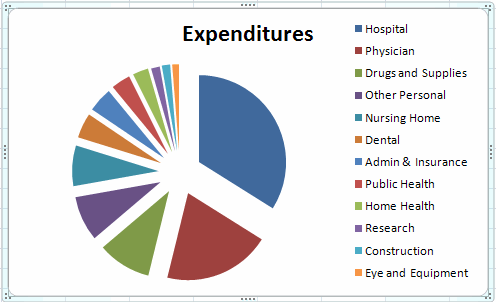
EXCEL Charts: Column, Bar, Pie and Line

› 07 › 09Rotate charts in Excel - spin bar, column, pie and line charts Jul 09, 2014 · After being rotated my pie chart in Excel looks neat and well-arranged. Thus, you can see that it's quite easy to rotate an Excel chart to any angle till it looks the way you need. It's helpful for fine-tuning the layout of the labels or making the most important slices stand out. Rotate 3-D charts in Excel: spin pie, column, line and bar charts

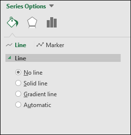
How To Use Dynamic Data Labels To Create Interactive Excel Charts

How to Add Two Data Labels in Excel Chart (with Easy Steps) 4 Quick Steps to Add Two Data Labels in Excel Chart. Step 1: Create a Chart to Represent Data. Step 2: Add 1st Data Label in Excel Chart. Step 3: Apply 2nd Data Label in Excel Chart. Step 4: Format Data Labels to Show Two Data Labels. Things to Remember.

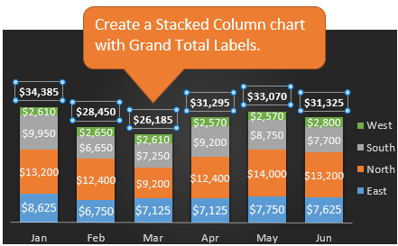
Create Dynamic Chart Data Labels with Slicers - Excel Campus

Excel: How to Create Chart & Ignore Blank Axis Labels This tutorial provides a step-by-step example of how to create a chart in Excel and ignore blank axis labels. Step 1: Enter Data with Some Blank Values. First, let's enter the following dataset into Excel that contains some blank values for the axis labels: If we highlight this range of data and insert a bar chart, the x-axis will have several blank values: Step 2: Modify the Data to Remove Blank Values

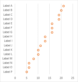
Dot Plots in Microsoft Excel - Peltier Tech Blog

Excel Gauge Chart Template - Free Download - How to Create Step #3: Rotate the doughnut chart. Next, you need to adjust the position of the chart to lay the groundwork for the future half-circle gauge. Right-click on the doughnut chart body and choose Format Data Series. In the pane that appears to the right, set the Angle of first slice to 270° and the Doughnut Hole Size value to 50%.

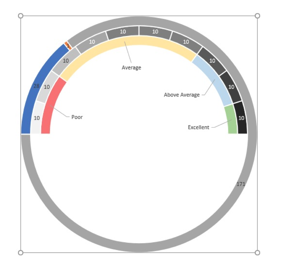
How To Build Gorgeous Speedometer Charts and Why You Shouldn't Use Them - I Will Teach You Excel

Data Labels in Excel Pivot Chart (Detailed Analysis) Then drag the Fill Handle first in the horizontal direction to cell H60. Next, drag the Fill Handle first in the vertical direction to cell H66. Then in a new sheet, create the following table as shown here, this table will help us to switch the Data Labels easily. From the Data Labels table, create a Pivot Chart.

Share :