41 excel pivot table conditional formatting row labels

How to Apply Conditional Formatting in Pivot Table? (with ... To apply conditional formatting in the pivot table, first, we must select the column to format. In this example, select "Grand Total Column." Then, in the "Home" Tab in the "Styles" section, click on "Conditional Formatting." Consequently, a dialog box pops up. Then, we need to click on "New Rule." As a result, another dialog box will pop up. Conditional formatting rows in a pivot table based on one ... I am havong difficulty trying to highlight an entire row in a pivot table based on one rows criteria. The pivot table is from A:M and I need to highlight the corresponding row if column I has 992 in it. I have tried sevral ways but can only get it to work if I just focus on one row. I am at a loss for what I am doing wrong.

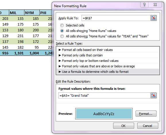
Conditional Format Pivot Table Row | Chandoo.org Excel ... Excel Ninja Apr 3, 2013 #2 Select the entire row, and when you apply the conditional format, make the column reference absolute. So, say we want the entire row 2 to be formatted if cell in col B = 5. formula would be: =$B2=5

Excel pivot table conditional formatting row labels

vba - Conditional Formatting in Pivot Table in Excel based ... In your pivot table, click in the values area ("Sum of Payment") in Cell B6, then select Home -->Conditional Formatting-->Manage Rules. Next "Add New Rule" and then make sure your rule looks like this: Create a second rule in the same manner and apply it to the pivot table. Share. Improve this answer. Apply conditional formatting for each row in Excel Then click Format button, in the Format Cells dialog, under Fill tab, select green color. Click OK > OK. 4. Then drag the AutoFill handle to adjacent rows which you want to apply the conditional rule to, then in select Fill Formatting Only from the Auto Fill Options. Sample File Click to download the sample file Design the layout and format of a PivotTable In the PivotTable Options dialog box, click the Layout & Format tab, and then under Layout, select or clear the Merge and center cells with labels check box. Note: You cannot use the Merge Cells check box under the Alignment tab in a PivotTable. Change the display of blank cells, blank lines, and errors

Excel pivot table conditional formatting row labels. 50 Things You Can Do With Excel Pivot Table | MyExcelOnline 18.07.2017 · A great way to highlight values within your data set, Excel Table or Pivot Table is to use Conditional Formatting rules. Formatting cells that contain a specific criteria, for example, greater than X or less than X, is a good way to visualize your results. When your criteria references a cell, then you can make this conditional format ... How to Apply Conditional Formatting to Pivot Tables ... So in this post I explain how to apply conditional formatting for pivot tables. 1. Select a cell in the Values area The first step is to select a cell in the Values area of the pivot table. If your pivot table has multiple fields in the Values area, select a cell for the field you want to apply the formatting to. 2. Apply Conditional Formatting Conditional Formatting on Pivot Table row labels In srcFromPowerPivot sheet cell A is from powerpivot under row label comparing the dates in cell C (3 dates) and the condtional formatting doesnt work. In cell J it worked cos I dragged under value instead of row label. In the srcFromWorksheet it worked even though it is under rowlabel. Sheet3 is just a copy of powerpivot data. 101 Advanced Pivot Table Tips And Tricks You Need To Know 25.04.2022 · Without a table your range reference will look something like above. In this example, if we were to add data past Row 51 or Column I our pivot table would not include it in the results. To create and name your table. Select your data. Go to the Insert tab and press the Table button in the Tables section, or use the keyboard shortcut Ctrl + T.

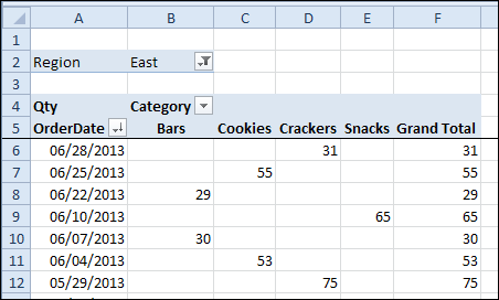
Pivot Table: Pivot table conditional formatting - Exceljet To apply conditional formatting to a pivot table, create a new conditional formatting rule and pay particular attention to the "apply rule to" settings as described below. In the example shown, there are two rules applied. The green shows the top 5 values using a rule like this: Details Excel tutorial: How to highlight rows with conditional ... To highlight rows in the table that contain tasks assigned to Bob, we need to take a different approach. First, select all of the data in the list. Then, choose New Rule from the conditional format menu on the Home tab of the ribbon. For style, choose "Classic". Then select "Use a formula to determine which cells to format". Format Pivot Table Labels Based on Date Range - Excel ... In the pivot table, remove any filters that have been applied - all the rows need to be visible before you apply the conditional formatting. Select all the dates in the Row Labels that you want to format. On the Ribbon, click the Home tab, and then in the Styles group, click Conditional Formatting. › pivot-tables › compare-listsHow To Compare Multiple Lists of Names with a Pivot Table Jul 08, 2014 · Column E of the Pivot Table contains the Grand Total (sum of columns B:D). People that volunteered all three years will have a “3” in column E. We should sort the pivot table so all the people with a “3” in column E appear at the top of the list. This will make it easier to find the names.

The Pivot table tools ribbon in Excel These two tabs allow you to perform pivot table customization. This is the Pivot table ribbon in Excel. Create pivot table fields , charts and sets. Here is an important thing to wonder for the pivot table ribbon in excel is as soon as you switch the selected cell to non pivot table cell. The pivot table ribbon disappears. So it means Excel ... FREE Online Excel Training (12+ Hours) | Learn Excel … Search and Highlight Data Using Conditional Formatting; Highlight Every Other Row in Excel; Highlight Blank Cells in Excel; Creating Heat Maps in Excel ; Here are some additional tutorials about Data Analysis: One Variable Data Table; Two Variable Data Table; Goal Seek in Excel; Scenario Manager in Excel; Using Solver in Excel; MODULE 5 - INTRODUCTION TO EXCEL … Conditional formatting for Pivot Tables in Excel 2016 ... The format I used was to select Conditional Formatting > Top 10 Items > set it to 1 item and select the default format. This format can be copied from one range to the next if desired or built up for each range individually. To copy the format, select one or more cells with that format and click Copy. How to Apply Conditional Formatting to Rows ... - Excel Campus On the Home tab of the Ribbon, select the Conditional Formatting drop-down and click on Manage Rules…. That will bring up the Conditional Formatting Rules Manager window. Click on New Rule. This will open the New Formatting Rule window. Under Select a Rule Type, choose Use a formula to determine which cells to format.

Re-Apply Pivot Table Conditional Formatting - yoursumbuddy

How to Apply Conditional Formatting to Pivot Tables - Excel … 13.12.2018 · Bottom Line: Learn how to apply conditional formatting to pivot tables so that the formats are dynamically reapplied as the pivot table is changed, filtered, or updated. Skill Level: Intermediate Download the Excel File. Here's the file that I use in the video. You can use it to practice adding, deleting, and changing conditional formatting on a variety of pivot table …

Design your Pivot Table in Excel | Excel in Excel

Conditional Format Pivot Table Cell based on another cell ... Hi there I am working on a pivot table that highlights cells based on a Min. Value. However I would like the ability to color code the conditional formatting based on the product which is listed in the product column... apple, turnip, carrot etc. Make the apple cell red, carrot orange etc. On a side note I originally created custom number formatting to the Row column table.

How to Apply Data Bars in Pivot Table - MS Excel | Excel In Excel

Pivot Table with Conditional Formatting - Microsoft Community Ok, Pivot Tables are good, Pivot Tables are our friends. Now I want to use conditional formatting with a pivot table. I have seen a lot of examples, but none showing me how to use a field in the field list in the formula of a conditional format. Perhaps this is not possible, so I moved the field into a row label.

How To Find And Remove Duplicates In A Pivot Table - MS Excel | Excel In Excel

How to Group Numbers in Pivot Table in Excel You May Also Like the Following Pivot Table Tutorials: How to Group Dates in Pivot Table in Excel. How to Create a Pivot Table in Excel. Preparing Source Data For Pivot Table. How to Refresh Pivot Table in Excel. Using Slicers in Excel Pivot Table – A Beginner’s Guide. How to Apply Conditional Formatting in a Pivot Table in Excel.

Format Pivot Table Labels Based on Date Range – Excel Pivot Tables

Apply Conditional Formatting | Excel Pivot Table Tutorial Steps to Apply Conditional Formatting to a Pivot Table. Applying conditional formatting in a pivot table seems tricky at first sight but actually, it's simple and easy. In the below pivot table, you need to apply "3-Color Scales" on "Month" values. Let's follow these steps.

How to Create a MS Excel Pivot Table – An Introduction | SIMPLE TAX INDIA

How to Create a Pivot Table in Excel: A Step-by-Step Tutorial 31.12.2021 · After you've completed Step 3, Excel will create a blank pivot table for you. Your next step is to drag and drop a field — labeled according to the names of the columns in your spreadsheet — into the Row Labels area. This will determine what unique identifier — blog post title, product name, and so on — the pivot table will organize ...

Sorting a Pivot Table - Free Microsoft Excel Tutorials

How to rename group or row labels in Excel PivotTable? 1. Click at the PivotTable, then click Analyze tab and go to the Active Field textbox. 2. Now in the Active Field textbox, the active field name is displayed, you can change it in the textbox. You can change other Row Labels name by clicking the relative fields in the PivotTable, then rename it in the Active Field textbox.

Share :