41 excel chart change labels

Excel Chart Data Labels-Modifying Orientation - Microsoft Community Replied on September 14, 2016 In reply to PaulaAB's post on September 13, 2016 Hi Paula, You can right click on the data label part then select Format Axis. Click on the Size & Properties tab then adjust the Text Direction or Custom Angle. Thanks, Mike Report abuse 6 people found this reply helpful · Was this reply helpful? Replies (7) editing Excel histogram chart horizontal labels - Microsoft Community editing Excel histogram chart horizontal labels. I have a chart of continuous data values running from 1-7. The horizontal axis values show as intervals [1,2] [2,3] and so on. I want the values to show as 1 2 3 etc. I have tried inserting a column of the values 1-7 alongside the data and selecting that as axis values; copying the data to a new ...

peltiertech.com › text-labels-on-horizontal-axis-in-eText Labels on a Horizontal Bar Chart in Excel - Peltier Tech Dec 21, 2010 · In Excel 2003 the chart has a Ratings labels at the top of the chart, because it has secondary horizontal axis. Excel 2007 has no Ratings labels or secondary horizontal axis, so we have to add the axis by hand. On the Excel 2007 Chart Tools > Layout tab, click Axes, then Secondary Horizontal Axis, then Show Left to Right Axis.

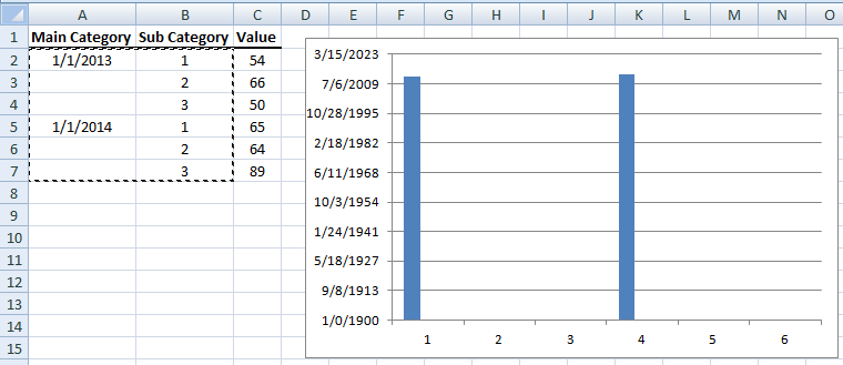
Excel chart change labels

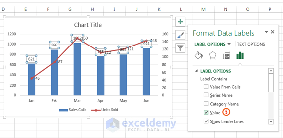
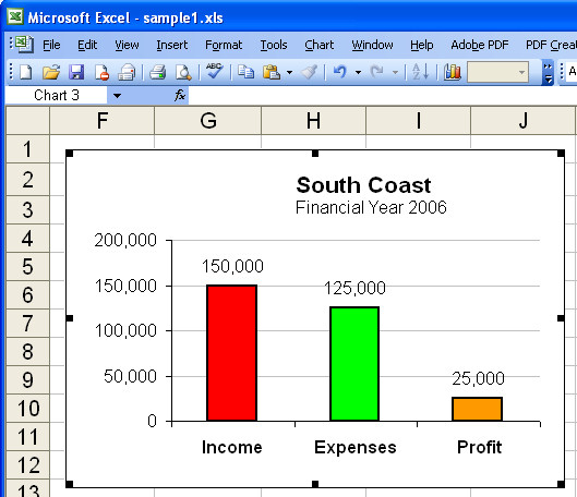
Add or remove data labels in a chart - support.microsoft.com Click the data series or chart. To label one data point, after clicking the series, click that data point. In the upper right corner, next to the chart, click Add Chart Element > Data Labels. To change the location, click the arrow, and choose an option. If you want to show your data label inside a text bubble shape, click Data Callout. chandoo.org › wp › change-data-labels-in-chartsHow to Change Excel Chart Data Labels to Custom Values? You can change data labels and point them to different cells using this little trick. First add data labels to the chart (Layout Ribbon > Data Labels) Define the new data label values in a bunch of cells, like this: Now, click on any data label. This will select "all" data labels. Now click once again. › documents › excelHow to change chart axis labels' font color and size in Excel? We can easily change all labels' font color and font size in X axis or Y axis in a chart. Just click to select the axis you will change all labels' font color and size in the chart, and then type a font size into the Font Size box, click the Font color button and specify a font color from the drop down list in the Font group on the Home tab.

Excel chart change labels. support.microsoft.com › en-us › topicChange axis labels in a chart - support.microsoft.com Your chart uses text from its source data for these axis labels. Don't confuse the horizontal axis labels—Qtr 1, Qtr 2, Qtr 3, and Qtr 4, as shown below, with the legend labels below them—East Asia Sales 2009 and East Asia Sales 2010. Change the text of the labels. Click each cell in the worksheet that contains the label text you want to ... Axis Label Alignment - Microsoft Community By default, they are at a 45 degree angle, and cut off with ... when too long. In older versions, I could right click, choose "Format axis", then change the alignment of the label. I see no such options in Excel 2016. All assistance I've found says there should be an alignment option under Axis Options. Excel charts: add title, customize chart axis, legend and data labels ... How to change data displayed on labels To change what is displayed on the data labels in your chart, click the Chart Elements button > Data Labels > More options… This will bring up the Format Data Labels pane on the right of your worksheet. Switch to the Label Options tab, and select the option (s) you want under Label Contains: Edit titles or data labels in a chart - support.microsoft.com The first click selects the data labels for the whole data series, and the second click selects the individual data label. Right-click the data label, and then click Format Data Label or Format Data Labels. Click Label Options if it's not selected, and then select the Reset Label Text check box. Top of Page

2/ Right-click i.e. on the 1st histo. bar (A) > Add Data Labels (numbers are displayed a the top of the bars) 3/ Click one of the numbers that just displayed (the Format Data Labels pane opens on the right) > Check option "Value From Cells" > Select range C2:C7 > OK > Uncheck option "Value" demo.png (18.5 KiB) · 3 › 509290 › how-to-use-cell-valuesHow to Use Cell Values for Excel Chart Labels Mar 12, 2020 · The values from these cells are now used for the chart data labels. If these cell values change, then the chart labels will automatically update. Link a Chart Title to a Cell Value. In addition to the data labels, we want to link the chart title to a cell value to get something more creative and dynamic. We will begin by creating a useful chart ... How to Create and Customize a Waterfall Chart in Microsoft Excel Select the chart and use the buttons on the right (Excel on Windows) to adjust Chart Elements like labels and the legend, or Chart Styles to pick a theme or color scheme. Select the chart and go to the Chart Design tab. Custom Data Labels with Colors and Symbols in Excel Charts - [How To] The chart will show the upward and downward arrow instantly. 1.1.1 Problems. Problem as I said in the beginning is that though the data labels I connected will update if data changes, but if I throw additional rows to the chart, the new data labels needs to be connected too and that makes it quite cumbersome.

How to rotate axis labels in chart in Excel? Go to the chart and right click its axis labels you will rotate, and select the Format Axis from the context menu. 2. In the Format Axis pane in the right, click the Size & Properties button, click the Text direction box, and specify one direction from the drop down list. See screen shot below: The Best Office Productivity Tools Is there a way to change the order of Data Labels? Microsoft Agent | Moderator Replied on April 4, 2018 Hi Keith, I got your meaning. Please try to double click the the part of the label value, and choose the one you want to show to change the order. Thanks, Rena ----------------------- * Beware of scammers posting fake support numbers here. How to Customize Your Excel Pivot Chart Data Labels - dummies The Data Labels command on the Design tab's Add Chart Element menu in Excel allows you to label data markers with values from your pivot table. When you click the command button, Excel displays a menu with commands corresponding to locations for the data labels: None, Center, Left, Right, Above, and Below. None signifies that no data labels should be added to the chart and Show signifies ... Create a column chart with percentage change in Excel Right click any one column bar in the chart, and then choose Change Series Chart Type from the context menu, see screenshot: 8. In the Change Chart Type dialog box, change both Increase and Decrease to Scatter chart, then uncheck the Secondary Axis box for each from Choose the chart type and axis for your series list box. See screenshot: 9.

Fixing Your Excel Chart When the Multi-Level Category Label Option is ...

How to Change the Y Axis in Excel - Alphr Click the dropdown next to "Display Units," then make your selection such as "millions" or "hundreds." To label the displayed units, go to the "Axis Options -> Display units" section. Add a...

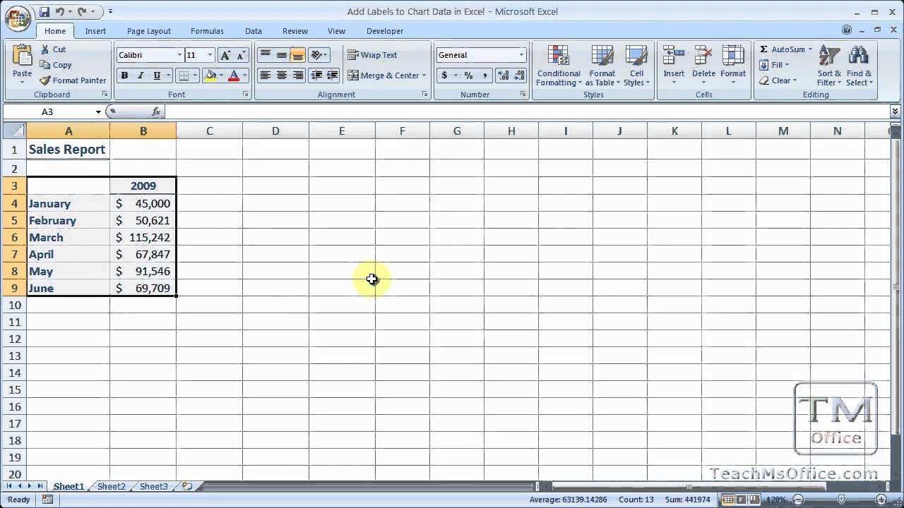
Add Labels to Chart Data in Excel - YouTube

How to edit the label of a chart in Excel? - Stack Overflow The latter box will list the "1", "2", etc. numbers that you want to change. Hit the edit button for the right-hand box (Horizontal Category (Axis) Labels), and you will be prompted to enter an axis label range. Instead of selecting a range, though, just enter the labels that you want to see on the x-axis, separated by commas, like so:

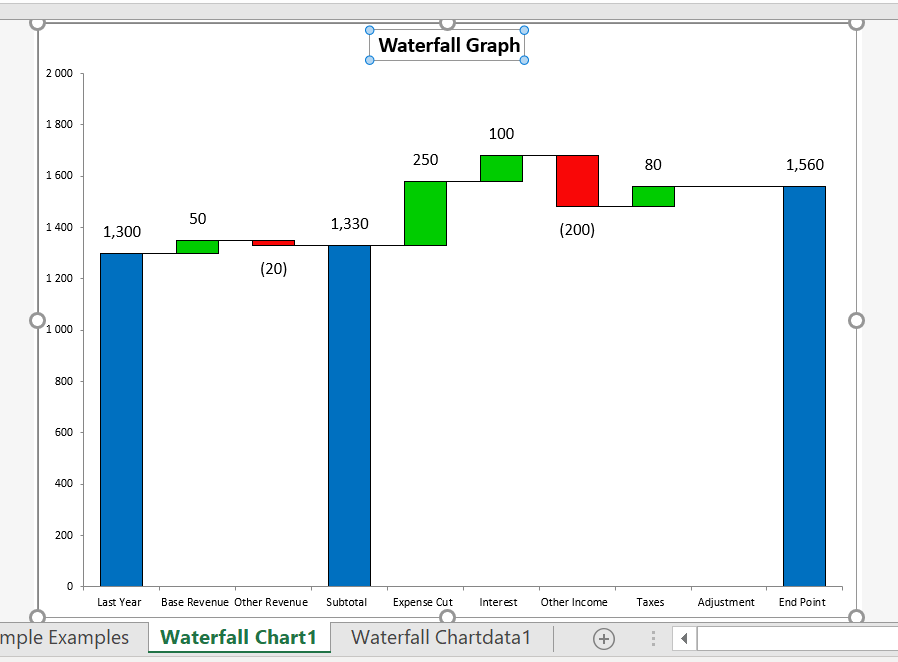
Waterfall Chart Templates (Excel 2010 and 2013) – Edward Bodmer ...

How to group (two-level) axis labels in a chart in Excel? The Pivot Chart tool is so powerful that it can help you to create a chart with one kind of labels grouped by another kind of labels in a two-lever axis easily in Excel. You can do as follows: 1. Create a Pivot Chart with selecting the source data, and: (1) In Excel 2007 and 2010, clicking the PivotTable > PivotChart in the Tables group on the ...

34 Label Chart In Excel - Labels Database 2020

Excel VBA Chart Data Label Font Color in 4 Easy Steps (+ Example) In this Excel VBA Chart Data Label Font Color Tutorial, you learn how to change a Chart's Data Label(s) font color with Excel macros.. This Excel VBA Chart Data Label Font Color Tutorial: Applies to Data Labels in a Chart. Doesn't apply to the following: ActiveX Labels in a worksheet.

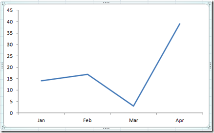
How-to Add Custom Labels that Dynamically Change in Excel Charts ...

Change axis labels in a chart in Office - support.microsoft.com To change the label, you can change the text in the source data. If you don't want to change the text of the source data, you can create label text just for the chart you're working on. In addition to changing the text of labels, you can also change their appearance by adjusting formats.

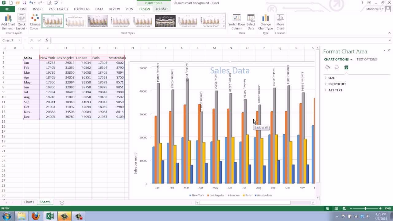
How to Add Data Labels to your Excel Chart in Excel 2013 - YouTube

Excel Custom Chart Labels • My Online Training Hub Using Excel custom chart labels is a great way to create a more insightful chart without having to show a whole other series. Just take this chart below with custom labels showing the year on year % change:

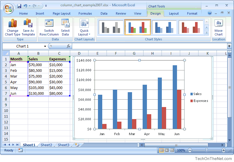
create excel spreadsheet for your data for $5 - SEOClerks

Excel tutorial: How to customize axis labels Instead you'll need to open up the Select Data window. Here you'll see the horizontal axis labels listed on the right. Click the edit button to access the label range. It's not obvious, but you can type arbitrary labels separated with commas in this field. So I can just enter A through F. When I click OK, the chart is updated.

Do My Excel Blog: How to design a multiple clustered bar chart series ...

› excel-chart-verticalExcel Chart Vertical Axis Text Labels • My Online Training Hub Label specific Excel chart axis dates to avoid clutter and highlight specific points in time using this clever chart label trick. Jitter in Excel Scatter Charts Jitter introduces a small movement to the plotted points, making it easier to read and understand scatter plots particularly when dealing with lots of data.

Do My Excel Blog: How to design a multiple clustered bar chart series ...

excel - Change horizontal axis labels in XY Scatter chart with VBA ... Note chart isn't interactive, ie, changing values in spreadsheet won't change chart! Sub Plot_Chart() Dim v(), r As Long, c As Long 'Create and use chart With ActiveSheet.Shapes.AddChart(xlLineMarkers).Chart 'Clear all series and legend While .SeriesCollection.Count .SeriesCollection(1).Delete Wend .Legend.Delete 'Iterate through rows and ...

Do My Excel Blog: How to hide the zero percent labels in an Excel pie chart

support.microsoft.com › en-us › officeChange the format of data labels in a chart To get there, after adding your data labels, select the data label to format, and then click Chart Elements > Data Labels > More Options. To go to the appropriate area, click one of the four icons ( Fill & Line , Effects , Size & Properties ( Layout & Properties in Outlook or Word), or Label Options ) shown here.

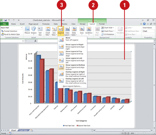
Microsoft Excel 2010 : Creating and Modifying Charts - Changing Chart ...

› documents › excelHow to change chart axis labels' font color and size in Excel? We can easily change all labels' font color and font size in X axis or Y axis in a chart. Just click to select the axis you will change all labels' font color and size in the chart, and then type a font size into the Font Size box, click the Font color button and specify a font color from the drop down list in the Font group on the Home tab.

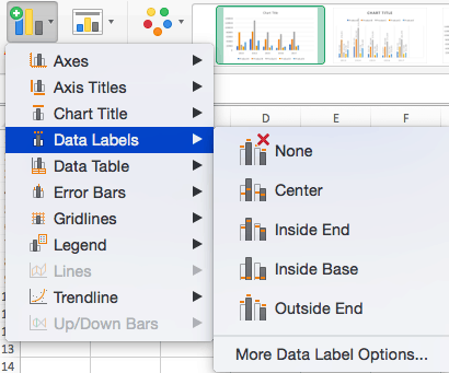
How to Make Charts and Graphs in Excel | Smartsheet

chandoo.org › wp › change-data-labels-in-chartsHow to Change Excel Chart Data Labels to Custom Values? You can change data labels and point them to different cells using this little trick. First add data labels to the chart (Layout Ribbon > Data Labels) Define the new data label values in a bunch of cells, like this: Now, click on any data label. This will select "all" data labels. Now click once again.